12 most useful Google Sheets functions

It's not a secret that there are tens of functions in spreadsheets, each with its own features and for its own purpose. But this doesn't mean you know nothing about electronic tables if you don't master them all.

There's a small set of Google Sheets functions that will let you last long enough without digging dip into spreadsheets. Allow me to introduce them to you.

Tip. If your task is super tricky and basic Google Sheets formulas are not what you're looking for, check out our collection of quick tools – Power Tools.

Google Sheets SUM function

Now, this is one of those Google Sheets functions that you have to learn one way or the other. It adds up several numbers and/or cells and returns their total:

=SUM(value1, [value2, ...])

value1 is the first value to sum. It can be a number, a cell with a number, or even a range of cells with numbers. This argument is required.
value2, ... – all other numbers and/or cells with numbers you'd like to add to value1. The square brackets hint that this one is optional. And in this particular case, it can be repeated several times.

Tip. You can find the functions among standard instruments on Google Sheets toolbar: Where to find SUM function.

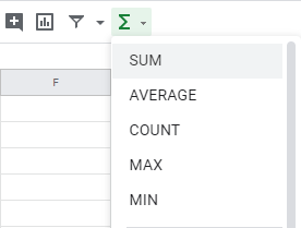
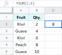
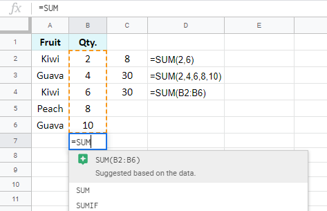
I can create various Google Sheets SUM formulas like these:

=SUM(2,6) to calculate two numbers (the number of kiwis for me) Calculate two numbers.

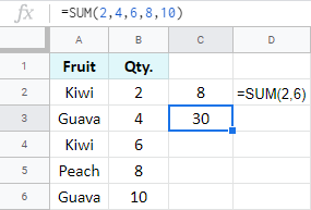
=SUM(2,4,6,8,10) to calculate several numbers Add multiple numbers directly within the formula.

=SUM(B2:B6) to add up multiple cells within the range Add up range in Google Sheets.

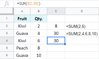
Tip. There's a trick the function lets you do in order to swiftly add cells in Google Sheets in a column or a row. Try entering the SUM function right below the column you want to total or to the right of the row of interest. You'll see how it suggests the correct range instantly: How to sum a column in Google Sheets.

COUNT & COUNTA

This couple of Google Sheets functions will let you know how many cells of different contents your range contains. The only difference between them is that Google Sheets COUNT works only with numeric cells, while COUNTA counts cells with text as well.

So, to total all cells with numbers only, you use COUNT for Google Sheets:

=COUNT(value1, [value2, ...])

value1 is the first value or range to check.
value2 – other values or ranges to use for counting. As I told you before, square brackets mean that the function may get by without value2.

Here's the formula I've got:

=COUNT(B2:B7) How to count in Google Sheets.

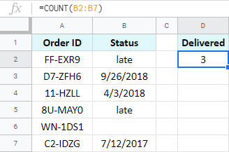
If I am to get all orders with a known status, I will have to use another function: COUNTA for Google Sheets. It counts all non-empty cells: cells with text, numbers, dates, booleans – you name it.

=COUNTA(value1, [value2, ...])

The drill with its arguments is the same: value1 and value2 represent values or ranges to process, value2 and the following are optional.

Notice the difference:

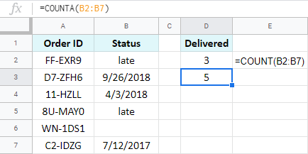
=COUNTA(B2:B7) Google Sheets: count non-empty cells.

COUNTA in Google Sheets takes all cells with contents into account, whether numbers or not.

SUMIF & COUNTIF

Whilst SUM, COUNT, and COUNTA calculate all records you feed to them, SUMIF and COUNTIF in Google Sheets process those cells that meet specific requirements. The parts of the formula will be as follows:

=COUNTIF(range, criterion)

range to count – required
criterion to consider for counting – required

=SUMIF(range, criterion, [sum_range])

range to scan for values related to the criterion – required
criterion to apply to the range – required
sum_range – the range to add up records from if it differs from the first range – optional

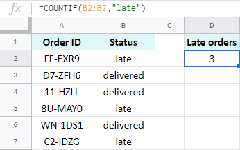
For example, I can find out the number of orders that fall behind schedule:

=COUNTIF(B2:B7,"late") Count orders based on criteria.

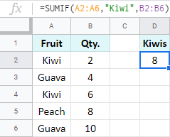
Or I can get the total quantity of kiwis only:

=SUMIF(A2:A6,"Kiwi",B2:B6) Sum numbers based on criteria.

Google Sheets AVERAGE function

In math, the average is the sum of all numbers divided by their count. Here in Google Sheets the AVERAGE function does the same: it evaluates the entire range and finds the average of all numbers ignoring the text.

=AVERAGE(value1, [value2, ...])

You can type in multiple values or/and ranges to consider.

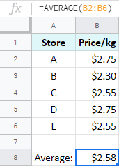
If the item is available for purchase in different stores at different prices, you can tally the average price:

=AVERAGE(B2:B6) Google Sheets AVERAGE formula.

Google Sheets MAX & MIN functions

The names of these miniature functions speak for themselves.

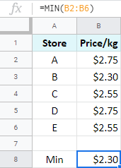
Use Google Sheets MIN function to return the minimum number from the range:

=MIN(B2:B6) Get the minimum price from the range.

Tip. To find the lowest number ignoring zeros, put the IF function inside:

=MIN(IF($B$2:$B$6<>0,$B$2:$B$6))

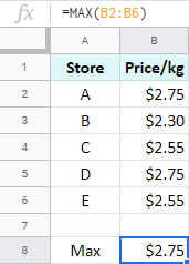
Use Google Sheets MAX function to return the maximum number from the range:

=MAX(B2:B6) Get the maximum price from the range.

Tip. Want to ignore zeros here as well? Not a problem. Just add another IF:

=MAX(IF($B$2:$B$6<>0,$B$2:$B$6))

Easy peasy lemon squeezy. :)

Google Sheets IF function

Though IF function in Google Sheets is quite popular and commonly used, for some reasons it keeps confusing and puzzling its users. Its main purpose is to help you work out conditions and return different results accordingly. It is also often referred to as Google Sheets "IF/THEN" formula.

=IF(logical_expression, value_if_true, value_if_false)

logical_expression is the condition itself that has two possible logical outcomes: TRUE or FALSE.
value_if_true is whatever you want to return if your condition is met (TRUE).
otherwise, when it's not met (FALSE), value_if_false is returned.

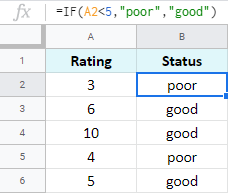
Here's a plain example: I'm evaluating ratings from feedback. If the number received is less than 5, I want to label it as poor. But if the rating is greater than 5, I need to see good. If I translate this to the spreadsheet language, I'll get the formula I need:

=IF(A6<5,"poor","good") IF function for Google Sheets.

AND, OR

These two functions are purely logical.

Google spreadsheet AND function checks if** all its values** are logically correct, while Google Sheets OR function – if any of the provided conditions are true. Otherwise, both will return FALSE.

To be honest, I don't remember using these much on their own. But both are used in other functions and formulas, especially with the IF function for Google Sheets.

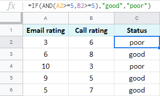
Adding Google Sheets AND function to my condition, I can check ratings in two columns. If both numbers are greater than or equal to 5, I mark the total request as "good", or else "poor":

=IF(AND(A2>=5,B2>=5),"good","poor") AND in the logic of the IF function.

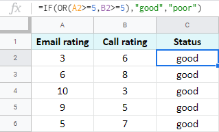
But I can also change the condition and mark the status good if at least one number of two is more than or equal to 5. Google Sheets OR function will help:

=IF(OR(A2>=5,B2>=5),"good","poor") OR in combination with IF.

CONCATENATE in Google Sheets

If you need to merge records from several cells into one without losing any of the data, you should use Google Sheets CONCATENATE function:

=CONCATENATE(string1, [string2, ...])

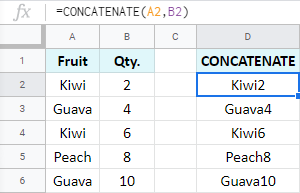
Whatever characters, words, or references to other cells you give to the formula, it will return everything in one cell:

=CONCATENATE(A2,B2) Merge cells in Google Sheets.

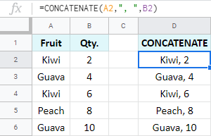
The function also lets you separate combined records with chars of your choice, like this:

=CONCATENATE(A2,", ",B2) Combine cells using delimiters.

Google Sheets TRIM function

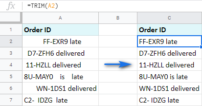
You can quickly check the range for any extra spaces using the TRIM function:

=TRIM(text)

Enter the text itself or a reference to a cell with text. The function will look into it and not only trim all leading and trailing spaces but will also reduce their number between words to one: Trim leading, trialling and extra spaces in Google Sheets.

TODAY & NOW

In case you work with daily reports or need today's date and the current time in your spreadsheets, TODAY and NOW functions are at your service.

With their help, you will insert today's date and time formulas in Google Sheets and they will update themselves whenever you access the document. I truly cannot imagine the simplest function than these two:

=TODAY() will show you the today's date.
=NOW() will return both the today's date and the current time.

Insert today's date in Google Sheets.

Google Sheets DATE function

If you're going to work with dates in electronic tables, Google Sheets DATE function is a must-learn.

When building different formulas, sooner or later you will notice that not all of them recognize dates entered as they are: 12/8/2019.

Besides, the locale of the spreadsheet dictates the format of the date. So the format you're used to (like 12/8/2019 in the US) may not be recognized by other users' Sheets (e.g. with the locale for the UK where dates look like 8/12/2019).

To avoid that, it's highly recommended to use the DATE function. It converts whatever day, month, and year you enter into a format that Google will always understand:

=DATE(year, month, day)

For example, if I were to subtract 7 days from my friend's birthday to know when to start preparing, I'd use the formula like this:

=DATE(2019,9,17)-7

Or I could make the DATE function return the 5th day of the current month and year:

=DATE(YEAR(TODAY()),MONTH(TODAY()),5)

Google Sheets VLOOKUP

And finally, the VLOOKUP function. That same function that keeps lots of Google Sheets users in terror. :) But the truth is, you only need to break it down once – and you won't remember how you lived without it.

Google Sheets VLOOKUP scans one column of your table in search of a record you specify and pulls the corresponding value from another column from that same row:

=VLOOKUP(search_key, range, index, [is_sorted])

search_key is the value to look for
range is the table where you need to search
index is the number of the column where related records will be pulled from
is_sorted is optional and used to hint that the column to scan is sorted

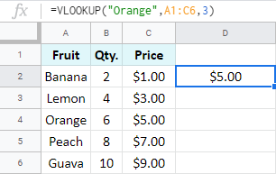
I have a table with fruits and I want to know how much oranges cost. For that, I create a formula that will look for Orange in the first column of my table and return the corresponding pricing from the third column:

=VLOOKUP("Orange",A1:C6,3) How to use the VLOOKUP function in Google Sheets.

Modify multiple Google Sheets formulas quickly with a special tool

We also have a tool that helps you modify multiple Google Sheets formulas within the selected range at once. It's called Formulas. Let me show you how it works.

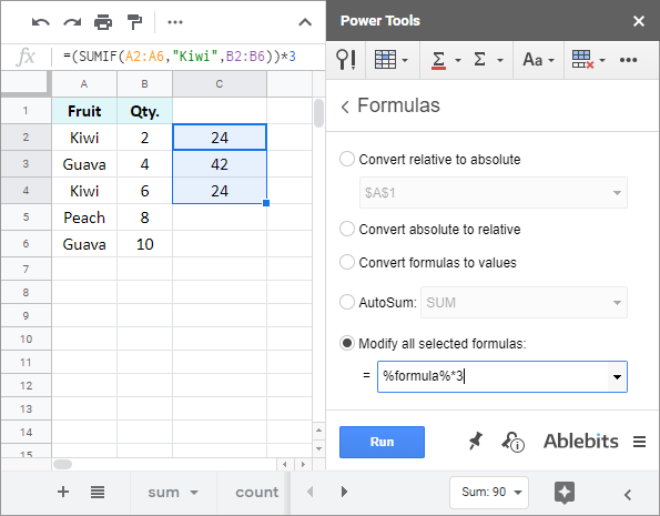
I have a small table where I used SUMIF functions to find the total of each fruit: My small table with fruits.

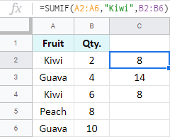
I want to multiply all totals by 3 to restock. So I select the column with my formulas and open the add-on.

Note. Since the utility is part of Power Tools, you need to install it first. You will find the tool right at the bottom of the pane: Formulas tool in Power Tools.

Then I choose the option to Modify all selected formulas, add *3 at the end of the formula sample, and click Run. You can see how the totals change accordingly – all in one go: Modify all formulas at once.

I hope this article has answered some of your questions about Google Sheets functions. If you have any other Google Sheets formulas in mind that haven't been covered here, let us know in comments below.

12 most useful Google Sheets functions